Skip to content

Category

small language model

343 papers

#small language model Open access Aug 2026

Only the Logarithm Adds ── +50% Followed by -50% Is Not 0% but -25% ── Repeating +/-10% Fifty Times Each Gives -39.50%, While the Naive Sum Answers 0% ── [Paper 292]

A “rate of return” looks like a quantity that can be added. This paper asks which way of writing it can──the answer is the log return alone. No new mathematical theorem and no new law is claimed. Scope of this paper (scope note): No new mathematical theorem and no new law is claimed──the relation between simple and log returns, the geometric mean, volatility drag, and the sqrt(n) rule are all standard. We do not build financial theory──all we use is one logarithm and one square root. We do not forecast prices──future returns and expectations are not treated at all. Only the composition rule for a given series is treated. We do not enter the tails──Paper 190 treated heavy tails and large deviations. This paper assumes no distributional shape and asks only whether addition is permitted. We do not hide the premise of the sqrt(n) rule──the sqrt(252) of Section 6 assumes independence between periods. With correlation it fails. We do not say sigma^2/2 is exact──as Section 4 shows, it is off by 7.18% at +/-50%. It is an approximation for small fluctuations. We give no investment advice──which mean to use depends on the question. This paper only separates which one answers what. Relation to earlier papers: Paper 194 showed that the four means are one family with only one fence of equality──that paper concerns the structure of the inequality at one instant; this one concerns which is right when composing along time, the same four means as material with orthogonal questions. Paper 132 showed that the 2 in Ito’s lemma is not a dimension──the sigma^2/2 here is that correction term itself, and the convergence table of Section 4 shows it numerically. Paper 190 measured “rare” on a logarithmic scale──here too one can add only after moving to the logarithm. Paper 272 showed that one and the same “twice” opens by 6.70 on the stimulus side──this paper is likewise about on which scale one adds. What is added is confirming that exponentiating the sum of logs leaves a difference of 0, lining up the three “averages” numerically, building a table in which the ratio to sigma^2/2 converges to 1.000025 as the fluctuation shrinks, and computing that +/-10% fifty times each gives -39.50%. First, we check on the smallest example.+50% then -50% sums to 0% in simple returns, but is actually -25% (Section 2). Second, this is the core of the paper. Exponentiating the sum of log returns ln1.5+ln0.5=-0.287682 gives 0.750000──the difference from the measured value is 0 (Section 2). Third, “average” names three different operations. Arithmetic mean 0%, geometric mean -13.3975%, exponentiated log mean -13.3975% (Section 3). Fourth, the gap is approximated by sigma^2/2. At +/-50% it is 12.5% against 13.3975%, an error of 7.18%; at +/-1% the ratio is 1.000025 (Section 4). Fifth, it bites over long series.+/-10% fifty times each gives -39.50%, while the naive sum answers 0% (Section 5). Sixth, annualisation is not addition either. A daily sigma=1% is 15.8745% a year, and multiplying by 252 overstates it by 15.87 times (Section 6). Returns do not add. Only the logarithm adds.+50% then -50% sums to 0% in simple returns but is actually -25%, while exponentiating the sum of logs, -0.287682, gives 0.750000 with a difference of 0. The single word “average” also names three operations──arithmetic 0%, geometric -13.3975%, and the geometric mean is nothing but the arithmetic mean of the logarithms (difference 10^-16). That gap is approximated by sigma^2/2, and shrinking the fluctuation from +/-50% to +/-1% takes the ratio from 1.0718 to 1.000025──the shape of Ito’s correction term, appearing in the numbers. And it bites over long series──+/-10% fifty times each, equal numbers of rises and falls, gives -39.4994%, and the naive sum answers 0%. One thing separates them──whether that quantity composes by multiplication or by addition. If by multiplication, move to logarithms and add there. If dispersion, move to variances and add there. What is added without moving is neither a return nor an average. On the making of this work: The ideas and content of this work stem from the author's own considerations. Assistance from an AI (a large language model) was used for structuring, English translation, and checking the algebra. Any remaining errors or misinterpretations are solely the author's. Feedback and corrections are sincerely appreciated. ----- 「収益率」は足し算できる量に見える。本稿が問うのは、どの書き方なら足せるかである──答は、対数収益率だけである。新しい数学定理も新しい法則も主張しない。 本稿の射程(射程注記):新しい数学定理も新しい法則も主張しない──単純収益率と対数収益率の関係、幾何平均、ボラティリティ・ドラッグ、sqrt(n) 則は、いずれも標準的である。金融理論を作らない──使うのは一つの対数と、一つの平方根だけである。価格を予測しない──将来の収益率も、期待値も一切扱わない。与えられた系列の合成規則だけを扱う。裾に入らない──論文190 が重い裾と大偏差を扱った。本稿は分布の形を一切仮定せず、足し算の可否だけを問う。 sqrt(n) 則の前提を隠さない──第6節の sqrt(252) は各期の独立性を仮定している。相関があれば成り立たない。 sigma^2/2 を厳密だと言わない──第4節が示すとおり、+/-50% では 7.18% ずれる。小さい変動での近似式である。投資助言をしない──どの平均を使うべきかは問いによる。本稿はどれが何を答えるかを分けるだけである。既刊との関係:論文194 は四つの平均が一つの族であり、等号の柵が一つしかないことを示した──あちらは一時点での不等式の構造、本稿は時間方向に合成したとき、どれが正しいかであり、同じ四つの平均を材料にして問いが直交している。論文132 は伊藤の 2 が次元ではないと示した──本稿の sigma^2/2 はその補正項そのものであり、第4節の収束表がそれを数で見せる。論文190 は「稀」を対数の目盛りで測った──本稿も対数に移してはじめて足せる。論文272 は同じ「二倍」が刺激の側で 6.70 倍ひらくことを示した──本稿もどの目盛りで足すかの問題である。加えたのは対数の和を指数に戻すと実測との差が 0 になると確かめたこと、三つの「平均」を数で並べたこと、sigma^2/2 が変動の縮小とともに比 1.000025 に収束する表を作ったこと、+/-10% を 50 回ずつで -39.50% になると計算したことである。 第一に、最小の例で確かめる。+50% のあと -50% は、単純収益率の和では 0% だが、実際は -25% である(第2節)。 第二に、これが本稿の芯である。対数収益率の和 ln1.5+ln0.5=-0.287682 を指数に戻すと 0.750000──実測との差は 0 である(第2節)。 第三に、「平均」が三つの別の操作を指す。算術平均 0%、幾何平均 -13.3975%、対数平均の指数 -13.3975%(第3節)。 第四に、差は sigma^2/2 で近似できる。+/-50% では 12.5% 対 13.3975% で 7.18% の誤差だが、+/-1% では比が 1.000025 になる(第4節)。 第五に、長い系列で効く。+/-10% を 50 回ずつで -39.50%、素朴な和は 0% と答える(第5節)。 第六に、年率換算も足し算ではない。日次 sigma=1% は年率 15.8745% であり、252 倍では 15.87 倍の過大評価になる(第6節)。 収益率は足せない。足せるのは対数だけである。+50% のあと -50% は、単純収益率の和では 0% だが実際は -25%であり、対数の和 -0.287682 を指数に戻すと 0.750000 で、実測との差は 0 になる。「平均」という一語も三つの操作を指す──算術平均 0%、幾何平均 -13.3975%、そして幾何平均は対数の算術平均に他ならない(差 10^-16)。その差は sigma^2/2 で近似でき、変動を +/-50% から +/-1% に縮めると比が 1.0718 から 1.000025 になる──伊藤の補正項の形が、数の上に現れる。そして長い系列で効く──+/-10% を 50 回ずつ、上げと下げが同じ回数なのに -39.4994% であり、単純な和は 0% と答える。分けるものは一つ──その量の合成が掛け算か、足し算か。掛け算なら対数に移してから足す。ばらつきなら分散に移してから足す。移さずに足したものは、収益率でも平均でもない。 作成にあたって:本稿の着想と内容は、著者自身の考察に基づくものです。文章の構成整理や英訳、数式の確認には AI(大規模言語モデル)の助力を得ました。最終的な内容の解釈や誤りがあれば、それらはすべて著者の責に帰します。お気づきの点があれば、ご教示いただければ幸いです。

Yuuki Yamagishi · 0 citations
#small language model Open access Aug 2026

"Capacity" Is a Number Attainable Only at Infinite Length ── At Blocklength 100 Only 41.68% of the Capacity Is Usable, and Reaching 99.99% Takes 3.4x10^9 ── C Is a Supremum, Not a Maximum ── [Paper 304]

Shannon’s coding theorem says that below the channel capacity C the error can be made arbitrarily small. This paper asks whether C itself is attainable──the answer is not at any finite blocklength. No new mathematical theorem and no new law is claimed. Scope of this paper (scope note): No new mathematical theorem and no new law is claimed──Shannon’s coding theorem, the capacity of the binary symmetric and Gaussian channels, and the finite-blocklength normal approximation are all standard. We do not build information theory──all we use is one binary entropy and one square root. We do not prove the coding theorem──achievability and the converse are merely quoted. We construct no codes──which codes approach capacity is not treated at all. Paper 163’s existence-versus-construction distinction is alive here too. We claim no accuracy for the normal approximation──R(n,epsilon)approx C-sqrt(V/n) Q^-1(epsilon) is a second-order approximation and errs appreciably at small n. The 41.68% at n=100 is an estimate, not an exact achievable rate. We do not discuss implementation──decoding effort, latency, and the performance of real codes are not treated. We do not criticise C──being a supremum is not a defect. Unattainable and meaningless are different. We fix one channel──Sections 3 and 4 are numbers for the single channel BSC(p=0.11). Other channels have other V and need other n. Relation to earlier papers: Paper 252 counted four quantities called “information,” needing different things──the C here is one of them (a supremum of mutual information), and its attainment is questioned. Paper 294 showed that separation improves only as the square root of length──the 1/sqrt(n) here comes from the same root (the additivity of variance). Paper 163 separated “a good code exists” from “here is a good code”──this paper treats a third: how long it must be. Paper 302 treated how existence does not give quantity──here quantity can be answered, and the answer was infinity. What is added is computing that only 41.68% of capacity is usable at n=100, giving the n required for 99% and 99.99% as 3.4x10^5 and 3.4x10^9, confirming that the loss falls as 1/sqrt(n), and placing as the separator that C is a supremum and not a maximum. First, capacity is fixed by the error rate. For the binary symmetric channel C=1-h(p), and C=0 at p=0.5 (Section 2). Second, this is the core of the paper. At blocklength n=100, only 41.68% of the capacity is usable (Section 3). Third, reaching 99% takes n=3.4x10^5. Reaching 99.99% takes 3.4x10^9 (Section 3). Fourth, the loss falls only as 1/sqrt(n). Multiply n by 100 and the loss is one tenth (Section 4). Fifth, C is not a maximum. R=C is attained at no n, and only as n->infinity does R-> C (Section 5). Sixth, the separator is an attained maximum against an unattained supremum (Section 6). Shannon’s coding theorem says that below C the error can be made arbitrarily small. But C itself is attained at no finite blocklength. Counting on BSC(p=0.11) at error 10^-3: at blocklength 100 only 41.68% of the capacity is usable──99% takes 3.401x10^5, and 99.99% takes 3.4x10^9, a codeword of 3.4 billion bits. The loss falls only as 1/sqrt(n)──multiplying n by 100 divides the loss by 10, from the same root (the additivity of variance) by which Paper 294 measured separation. And at every finite n the loss is positive──C is not the maximum of the set of achievable rates but its supremum. One thing separates them──whether the number belongs to the set or not. Say “a channel of capacity C” and still no device sending C bits exists. What exists is only the fact that devices arbitrarily close to C can be built. On the making of this work: The ideas and content of this work stem from the author's own considerations. Assistance from an AI (a large language model) was used for structuring, English translation, and checking the algebra. Any remaining errors or misinterpretations are solely the author's. Feedback and corrections are sincerely appreciated. ----- シャノンの符号化定理は、通信路容量 C より低い速度なら誤りを任意に小さくできると言う。本稿が問うのは、C そのものは達成できるかである──答は、どんな有限の符号長でも達成できないである。新しい数学定理も新しい法則も主張しない。 本稿の射程(射程注記):新しい数学定理も新しい法則も主張しない──シャノンの符号化定理、二元対称通信路の容量、ガウス通信路の容量、有限長の正規近似は、いずれも標準的である。情報理論を作らない──使うのは一つの二値エントロピーと、一つの平方根だけである。符号化定理を証明しない──到達性も逆定理も引くだけである。符号を構成しない──どの符号が容量に近づくかは一切扱わない。論文163 の「存在と構成」の区別が、ここでも生きている。正規近似の精度を主張しない──R(n,epsilon)approx C-sqrt(V/n) Q^-1(epsilon) は第二次の近似であり、n が小さいところでは誤差が大きい。 n=100 の 41.68% は目安であって、厳密な達成可能速度ではない。実装を論じない──復号の手間も、遅延も、実際の符号の性能も扱わない。 C を批判しない──上限であることは欠陥ではない。達成されないことと、意味がないことは違う。通信路を一つに絞る──第3・4節はBSC(p=0.11) という一つの通信路での数である。他の通信路では V が変わり、必要な n も変わる。既刊との関係:論文252 は「情報量」が四つあり要るものが違うと数えた──本稿の C はそのうちの一つ(相互情報量の上限)であり、達成条件を問う。論文294 は分離が長さの平方根でしか良くならないと示した──本稿の 1/sqrt(n) は同じ根(分散の加法性)から来る。論文163 は「良い符号が在る」と「これが良い符号だ」を分けた──本稿は三つ目、「どれだけ長ければ良いか」を扱う。論文302 は存在が定量を教えないことを扱った──本稿は定量が答えられる場合であり、答が「無限」だった。加えたのはn=100 で容量の 41.68% しか使えないと計算したこと、99%/99.99% に要る n を 3.4x10^5/3.4x10^9 と出したこと、損失が 1/sqrt(n) で減ると確かめたこと、C が上限であって最大値でないと分離子に据えたことである。 第一に、容量は誤り率から決まる。二元対称通信路で C=1-h(p) であり、p=0.5 で C=0 になる(第2節)。 第二に、これが本稿の芯である。符号長 n=100 では、容量の 41.68% しか使えない(第3節)。 第三に、99% に届くには n=3.4x10^5 が要る。99.99% なら 3.4x10^9 である(第3節)。 第四に、損失は 1/sqrt(n) でしか減らない。 n を 100 倍にして、損失は 10 分の一である(第4節)。 第五に、C は最大値ではない。 R=C ちょうどはどの n でも達成されず、n->infinity ではじめて R-> C になる(第5節)。 第六に、分離子は「達成される最大値か、達成されない上限か」である(第6節)。 シャノンの符号化定理は「R

Yuuki Yamagishi · 0 citations
#large language models Open access Aug 2026

Executable Memory and World Coupling: Code as Cognitive Interface in a Self-Modifying Simulation

【Version note — v3】This version removes all literature citations; the Related Work section now states explicitly that the work is bottom-up and experiment-driven, and that we prefer an explicit statement of independence over a performative reference list. Earlier versions (v1, v2) contain incomplete reference lists and should be treated as working drafts; the current version supersedes them. Large language model (LLM) agents have recently explored executable memory—compiling agent memory into code snippets that an external LLM interprets at inference time. We argue that this paradigm remains tied to a single architectural choice: the executor is an external model, the memory is a personal profile, and the code never participates in the agent's own memory economy. We present a cognitive simulation engine in which executable code is stored as unit-level memory entries and executed by a deterministic rule engine inside the simulation itself. A memory entry carrying an EXPR: prefix is a small program—an arithmetic expression over engine parameters and state variables—interpreted each generation; its result feeds directly into the unit's behavioral circuits. Code memory participates in the engine's memory economy: entries decay, are reinforced by hits, are evicted by capacity limits, and pass the same verification gates as any mechanism. Units acquire executable fragments by foraging, coupling energy gain with behavioral information transfer. Experiments show that (i) code memory measurably alters survival dynamics (extinction-count growth reduced by roughly 97% at threat 1.0); (ii) the survival benefit of code is stratified by strategy—decay reinforcement confers +15 generations at threat 1.5, healing reinforcement +10, while aggressive threat clearance confers no gain (clearing danger memories also clears the fear that drives defensive behavior); (iii) beyond a critical threat intensity (3.0) no code strategy confers benefit—a measured capability boundary; (iv) external trigger coupling: a unit's code can read an external trigger state (cognition) and, when the external signal is present, deterministically clear its own threat memories while writing an externally observable trace—with the external signal absent, the same code is inert, demonstrating that perception is a necessary component of the response; (v) cognitive code is acquired, not inherited: newly born units without the code fragment cannot perceive the external state, making cognition an evolvable individual trait; and (vi) when defensive and adversarial code coexist, an arms race emerges from primitive operations alone. We also report an unexpected semantics of negative-valued code, its diagnosis, and its redesign as a candidate inhibitory mechanism. The architecture points toward self-modifying systems in which memory, behavior, perception, and robustness converge on a single executable substrate.

Yizhang Hu · 0 citations
#small language model Dataset Open access Aug 2026

"Efficient Automated Mathematical Optimization with Supervisor-Guided Agentic SLMs: Base, CoT, and Agentic Datasets "

"This dataset supports research on automated mathematical optimization using specialized small language models (SLMs). It consists of 12 JSONL files, each containing 500 records, organized across four task-specific components: decision variables, objective functions, constraints, and CPLEX code generation. Each record follows an instruction\u2013input\u2013output structure, where the input contains a natural-language optimization problem and the output provides the corresponding task-specific formulation or executable solver code. Three dataset variants are provided for each task: Base, Chain-of-Thought (CoT), and Agentic. The Base variant uses direct task instructions, while the CoT and Agentic variants use structured reasoning-oriented instructions to guide task decomposition and formulation. The datasets are designed to support the training and evaluation of specialized language models for translating natural-language optimization problems into structured mathematical formulations and executable CPLEX models."

Layan Refai, Abdulraheem Tarabiah, Ali Al-Mosawi et al. · 0 citations
#large language models Open access Aug 2026

One Number Sets the Limit of Forecasting ── Each Extra Day Costs 1.5874 Times the Initial Accuracy ── Observe 10 Times More Precisely and You Gain Only 4.98 Days ── [Paper 289]

That a weather forecast cannot reach beyond a certain horizon is due neither to missing equations nor to slow computers. This paper asks what sets the limit──the answer is one number, the error doubling time tau_d. No new mathematical theorem and no new law is claimed. Scope of this paper (scope note): No new mathematical theorem and no new law is claimed──exponential error growth, the doubling time, the limit of predictability, and the value tau_dapprox 1.5 days are all standard. We do not build meteorology──all we use is one exponential and its inverse. We do not discuss chaos──the Lorenz equations, attractors, and bifurcations are not treated at all. We do not discuss numerical weather prediction──grid resolution, parameterisation, and data assimilation are not treated. We do not say the error grows exactly exponentially──e^lambda t holds only while the error is small, and growth stops near saturation. The computations here are confined to the linear-growth regime. We assert no value for tau_d──1.5 days is a representative value widely used in the literature, and it moves from about 1 to 2.5 days with season, region, and variable. Section 5 shows the size of that dependence itself. We do not say there is a single exponent──the real atmosphere has different growth rates at different scales, with smaller eddies growing faster. A single tau_d is a crude approximation. We do not deny that forecasts improve──forecasts have in fact grown longer. What this paper says is only that the growth is logarithmic, not that improvement is pointless. Relation to earlier papers: Paper 253 showed that time is one-dimensional because prediction demands it, not because a law says so──this paper turns how far that demand can be met into a number. Paper 195 separated “stable” into six words──that paper is a classification of stability; this one is a time scale of predictability, the same hyperbolicity as material with a different question. Paper 190 measured “rare” on a logarithmic scale──the return here is likewise logarithmic. Paper 266 showed that the premise of the sampling theorem is never met──“knowing the initial state exactly” here is likewise a premise never met, the same figure. What is added is writing the price per day as the fixed factor 1.5874, computing the accuracy needed for 14->21->30->60 days as 25.40 / 1625.5 / 1.70x10^9, writing backwards that 10 times the observation gains only 4.98 days, and sweeping tau_d from 1.0 to 2.5 to show the answer moving from 65536 to 84.4. First, the price per day is a fixed factor. With tau_d=1.5 days, each extra day costs 1.5874 times the initial accuracy (Section 2). Second, this is the core of the paper. Going from 14 to 21 days costs 25.40 times; to 30 days, 1625.5 times; to 60 days, 1.70x10^9 times (Section 2). Third, read backwards, the return is logarithmic. Observing 10 times more precisely gains only 4.98 days (Section 3). Fourth, even 10^9 times gains only 44.85 days (Section 3). Fifth, the familiar “about two weeks” comes from here. If the initial error is 10^-3 of saturation, the forecastable span is 14.95 days (Section 4). Sixth, the separator is tau_d itself. At tau_d=1.0 day the same extension costs 65536 times; at 2.5 days only 84.4──everything rides on one number (Section 5). What sets the limit of forecasting is neither the equations nor the computers, but one number, the error doubling time tau_d. At tau_d=1.5 days, each extra day costs 1.5874 times the initial accuracy──the factor is the same wherever the day is added, but the extension adds while the price multiplies, so one week costs 25.4, two weeks 645, six weeks 1.7 billion. Read backwards, observing 10 times more precisely gains only 4.98 days, and even 10^9 times gains 44.85. The familiar “about two weeks” comes from this one line──14.95 days at an initial error of 10^-3 of saturation. One thing separates them──tau_d itself. At 1.0 day the same extension costs 65536; at 2.5 days, 84.4. A factor of 776 arises from a single number. So the work of extending forecasts and the work of measuring tau_d carry the same weight. On the making of this work: The ideas and content of this work stem from the author's own considerations. Assistance from an AI (a large language model) was used for structuring, English translation, and checking the algebra. Any remaining errors or misinterpretations are solely the author's. Feedback and corrections are sincerely appreciated. ----- 天気予報がある日数より先を当てられないのは、方程式が足りないからでも、計算機が遅いからでもない。本稿が問うのは、何が限界を決めているかである──答は、誤差の二重時間 tau_d という一つの数である。新しい数学定理も新しい法則も主張しない。 本稿の射程(射程注記):新しい数学定理も新しい法則も主張しない──誤差の指数増大、二重時間、予測可能性の限界、tau_dapprox 1.5 日という値は、いずれも標準的である。気象学を作らない──使うのは一つの指数関数と、その逆関数だけである。カオスを論じない──ローレンツ方程式も、アトラクタも、分岐も一切扱わない。数値予報を論じない──格子解像度も、パラメタリゼーションも、データ同化も扱わない。誤差が厳密に指数増大すると言わない──e^lambda t が成り立つのは誤差が小さいあいだだけであり、飽和に近づけば増大は止まる。本稿の計算は線形増大の領域に限る。 tau_d の値を主張しない──1.5 日は文献で広く用いられる代表値であり、季節・領域・変数によって 1 日から 2.5 日程度まで動く。第5節はこの依存の大きさそのものを示す。単一の指数だと言わない──実際の大気には尺度ごとに違う成長率があり、小さい渦ほど速く育つ。単一の tau_d は粗い近似である。予報の改善を否定しない──現に予報は延びてきた。本稿が言うのはその延び方が対数的であるということだけであり、改善が無意味だとは言わない。既刊との関係:論文253 は時間が一本なのが法則ではなく「予言できる」という要求だと示した──本稿はその要求が、どこまでなら満たせるかを数にする。論文195 は「安定」が六つの別の言葉だと分けた──あちらは安定性の分類、本稿は予測可能性の時間尺度であり、同じ双曲性を材料にして問いが違う。論文190 は「稀」を対数の目盛りで測った──本稿の見返りも対数である。論文266 は標本化定理の前提が決して満たされないと示した──本稿の「初期値を正確に知る」も決して満たされない前提であり、構図が同じである。加えたのは一日あたりの代償を 1.5874 倍という一定倍率として書いたこと、14->21->30->60 日の必要精度を 25.40/1625.5/1.70x10^9 倍と計算したこと、観測 10 倍が 4.98 日にしかならないと逆から書いたこと、tau_d を 1.0 から 2.5 まで振って答が 65536 倍から 84.4 倍まで動くと示したことである。 第一に、一日ごとの代償は一定倍率である。 tau_d=1.5 日なら、一日延ばすたびに初期値の精度が 1.5874 倍要る(第2節)。 第二に、これが本稿の芯である。14 日を 21 日にするのに 25.40 倍、30 日にするのに 1625.5 倍、60 日にするのに 1.70x10^9 倍(第2節)。 第三に、逆から見ると見返りは対数的である。観測を 10 倍精密にしても、延びるのは 4.98 日だけである(第3節)。 第四に、10 億倍にしても 44.85 日である(第3節)。 第五に、約二週間という数がここから出る。初期誤差が飽和の 10^-3 なら、予報可能な期間は 14.95 日(第4節)。 第六に、分離子は「指数か多項式か」である。 tau_d を 1.0 日にすると同じ延長に 65536 倍要り、2.5 日なら 84.4 倍で済む──すべてが一つの数に乗っている(第5節)。 予報の限界を決めているのは、方程式でも計算機でもなく、誤差の二重時間 tau_d という一つの数である。 tau_d=1.5 日なら、一日延ばすたびに初期値の精度が 1.5874 倍要る──どこで延ばしても倍率は同じだが、延長は足し算で、代償は掛け算なので、一週間で 25.4 倍、二週間で 645 倍、一か月半で 17 億倍になる。逆から見れば、観測を 10 倍精密にしても延びるのは 4.98 日であり、10 億倍にしても 44.85 日である。よく言われる「約二週間」も、この一行から出る──初期誤差が飽和の 10^-3 なら 14.95 日。分けるものは一つ──tau_d そのもの。1.0 日なら同じ延長に 65536 倍要り、2.5 日なら 84.4 倍で済む。776 倍の違いが、たった一つの数から生まれる。だから予報を延ばす仕事と、tau_d を測る仕事は、同じ重さを持っている。 作成にあたって:本稿の着想と内容は、著者自身の考察に基づくものです。文章の構成整理や英訳、数式の確認には AI(大規模言語モデル)の助力を得ました。最終的な内容の解釈や誤りがあれば、それらはすべて著者の責に帰します。お気づきの点があれば、ご教示いただければ幸いです。

Yuuki Yamagishi · 0 citations
#large language models Open access Aug 2026

What Changed the Exponent of a Chain Was Self-Avoidance Alone, and above Four Dimensions That Cost Disappears ── An Error of 2.11% in the Exponent Becomes 29.33% in the Length at N=10^9 ── And 2+2=4 Empties Avoidance of Its Meaning ── [Paper 279]

The spread of a polymer chain is fixed by a power of the number of units N. For a Gaussian chain it is N^1/2, and for a self-avoiding chain N^0.588. This paper asks where that difference comes from and where it disappears──the answer is the count 2+2=4. No new mathematical theorem and no new law is claimed. Scope of this paper (scope note): No new mathematical theorem and no new law is claimed──the N^1/2 of a Gaussian chain, Flory's nu=3/(d+2), the exact three-dimensional value 0.58759, and that the upper critical dimension is 4 are all standard. No polymer physics is built──what is used is one power and a count of dimensions. Flory's formula is not derived──3/(d+2) is cited only, and the balance of free energies from which it comes is not entered. The 0.58759 is not computed──it is a cited value from numerical work and the renormalisation group. The renormalisation group is not entered──Papers 117 and 120 treat it. Rubber elasticity is not treated──an earlier candidate on forces holds the entropic force of a rubber band. This paper is confined to the exponent, not elasticity. Real polymers are not treated──neither solvent quality, nor stiffness, nor branching is treated. Only an idealised chain is examined. Flory's formula is not used at d>=4──it returns values below 0.5 and is outside its range. This paper writes that honestly. Relation to earlier papers: Paper 271 treated the upper critical dimension 4 of mean field──the 4 here is also an upper critical dimension, but in a different phenomenon (an Ising transition against the self-avoidance of a chain) at the same dimension. Paper 256 counted the range needed to tell two exponents apart──this paper counts the converse, how far a small error in an exponent is amplified in the length. Paper 144 read the exponent as the signature of what is conserved──the signature here is the constraint of self-avoidance. Paper 117 separated the four ways in which scale invariance fixes an exponent──the exponent here belongs to one of them, the fixed point. Paper 190 measured rare on a logarithmic scale──this paper likewise writes ratios in orders of magnitude. What is added is computing that an error of 2.11% in the exponent becomes 29.33% in the length at N=10^9, obtaining 10^11.42 as the N at which the ratio reaches 10, writing honestly that Flory's formula returns a physically impossible value at d=5, and writing the origin of the 4 as the count 2+2. First, set the two chains side by side. At N=10^6 the Gaussian chain gives 1000.0 and the self-avoiding chain 3353.8──a factor of 3.3538 (Section 2). Second, the gap keeps opening with N. At N=10^12 it is 11.2481, and the ratio reaches 10 at N=10^11.42 (Section 2). Third, this is the core of the paper. Flory's formula gives nu=0.6 against the exact 0.58759──an error of 2.11% in the exponent, which at N=10^9 becomes 29.33% in the length (Section 3). Fourth, the two coincide in four dimensions. Flory's 3/(d+2) is exactly 0.5000 at d=4──a difference of zero from the Gaussian chain (Section 4). Fifth, and there the formula ends its office. At d=5 it returns 0.4286, which falls below 0.5 and is physically impossible (Section 4). Sixth, the 4 comes out of a count. The images of two d-dimensional walks have dimensions summing to 2+2=4──above d=4 they do not meet in general position, so there is nothing to avoid (Section 5). what changed the exponent of the chain was one constraint alone, that it avoid itself. In three dimensions 0.5 becomes 0.58759, and at N=10^12 the lengths differ by 11.2481. And Flory's approximation, out by only 2.11% in the exponent, is out by 29.33% in the length at N=10^9──a small error inside a power is amplified with the orders of magnitude. But in four dimensions that difference disappears exactly. The reason is a count in geometry──the dimensions of two paths sum to 2+2=4, so for d>4 they do not meet in general position. The constraint did not disappear; what it constrained did. And there Flory's formula ends its office too──at d=5 it returns 0.4286, the impossible claim that a chain avoiding itself is more compact than one that does not. One thing separates them──confirming by a count whether the constraint still tells. Confirm it, and the range in which the formula may be used becomes clear. Do not confirm it, and one reads 0.4286 as a property of a chain. On the making of this work: The ideas and content of this work stem from the author's own considerations. Assistance from an AI (a large language model) was used for structuring, English translation, and checking the algebra. Any remaining errors or misinterpretations are solely the author's. Feedback and corrections are sincerely appreciated. ----- 高分子の鎖の広がりは、単位数 N の冪で決まる。ガウス鎖では N^1/2、自分を避ける鎖では N^0.588 である。本稿が問うのは、その差がどこから来て、どこで消えるのかである──答は、2+2=4 という数え上げである。新しい数学定理も新しい法則も主張しない。 本稿の射程(射程注記):新しい数学定理も新しい法則も主張しない──ガウス鎖の N^1/2、フローリーの nu=3/(d+2)、三次元の厳密値 0.58759、上部臨界次元が 4 であることは、いずれも標準的である。高分子物理を作らない──使うのは一つの冪と、次元の数え上げだけである。フローリーの式を導出しない──3/(d+2) を引くだけであり、自由エネルギーの平衡から出す議論には立ち入らない。0.58759 を計算しない──数値計算とくりこみ群による引用値である。くりこみ群に立ち入らない──論文117・120 が扱う。ゴム弾性を扱わない──第四波候補「力は六つあり」がゴム紐のエントロピー力を持つ。本稿は弾性ではなく指数に絞る。実在の高分子を扱わない──溶媒の良し悪しも、剛直性も、分岐も扱わない。理想化された鎖だけを見る。 d=5 以上でフローリーの式を使わない──0.5 を下回る値を返すので適用範囲の外である。本稿はこれを正直に書く。既刊との関係:論文271 は平均場の上部臨界次元が 4 であることを扱った──本稿の 4 も上部臨界次元だが、別の現象(イジングの相転移と、鎖の自己回避)で同じ次元が出ている。論文256 は二つの指数を見分けるのに要る範囲を数えた──本稿は逆に、指数のわずかな誤差が長さでどれだけ増幅されるかを数える。論文144 は指数を、何が保存しているかの署名として読んだ──本稿の署名は自己回避という束縛である。論文117 はスケール不変性が四通りに指数を選ぶことを分けた──本稿はその一つ(不動点)に属する指数を扱う。論文190 は「稀」を対数の目盛りで測った──本稿も比を桁で書く。加えたのは指数の 2.11% の誤差が N=10^9 の長さで 29.33% に増幅されると計算したこと、自己回避とガウスの比が 10 になる N を 10^11.42 と出したこと、d=5 でフローリーの式が物理的にありえない値を返すと正直に書いたこと、4 の出どころを 2+2 の数え上げとして書いたことである。 第一に、二つの鎖を並べる。 N=10^6 でガウス鎖は 1000.0、自己回避鎖は 3353.8──3.3538 倍である(第2節)。 第二に、差は N とともに開き続ける。 N=10^12 で 11.2481 倍、比が 10 になるのは N=10^11.42 である(第2節)。 第三に、これが本稿の芯である。フローリーの式は nu=0.6、厳密値は 0.58759──指数の誤差は 2.11% だが、N=10^9 の長さでは 29.33% になる(第3節)。 第四に、四次元で二つが一致する。フローリーの 3/(d+2) は d=4 でちょうど 0.5000──ガウス鎖と差がゼロになる(第4節)。 第五に、そこでフローリーの式は役目を終える。 d=5 では 0.4286 を返すが、これは 0.5 を下回るので物理的にありえない(第4節)。 第六に、4 の出どころは数え上げである。 d 次元の道二本の像は合わせて 2+2=4 次元──d>4 では一般の位置で交わらないので、避ける必要がそもそも生じない(第5節)。 鎖の指数を変えたのは、「自分を避ける」という束縛ただ一つであった。三次元では 0.5 が 0.58759 になり、N=10^12 では長さが 11.2481 倍違ってくる。そしてフローリーの近似は指数を 2.11% しか外さないのに、N=10^9 の長さでは 29.33% 外す──冪の中の小さな誤差は、桁とともに増幅される。だが四次元で、この差がちょうど消える。理由は幾何の数え上げである──二本の道の次元の和が 2+2=4 なので、d>4 では一般の位置で交わらない。束縛が消えたのではなく、束縛すべき相手が居なくなったのである。そしてそこでフローリーの式も役目を終える──d=5 で 0.4286 という、避ける鎖が避けない鎖より縮むというありえない値を返す。分けるものは一つ──束縛が効く場面かどうかを、数え上げで確かめること。確かめれば、式を使ってよい範囲が分かる。確かめなければ、0.4286 という値を鎖の性質として読んでしまう。 作成にあたって:本稿の着想と内容は、著者自身の考察に基づくものです。文章の構成整理や英訳、数式の確認には AI(大規模言語モデル)の助力を得ました。最終的な内容の解釈や誤りがあれば、それらはすべて著者の責に帰します。お気づきの点があれば、ご教示いただければ幸いです。

Yuuki Yamagishi · 0 citations
#large language models Dataset Open access Aug 2026

Police accountability data: United Kingdom, United States and Australia

Derived, machine-readable datasets on police complaints, stop and search, use of force and deaths following police contact, for the United Kingdom, the United States and Australia. Every figure is computed from official open data by code and published with its source, its period and its denominator attached. No figure was written, estimated or rounded by a language model. Where a rate cannot be computed honestly, the row is marked unpublishable with the reason recorded rather than being dropped. Contents. UK stop-and-search ethnic disparity by police force, computed as each ethnic group's share of recorded searches divided by that group's share of the force area's own resident population, joining data.police.uk to Census 2021 (TS021) via the ONS local-authority-to-police-force-area lookup, with a national summary; UK stop-and-search outcomes by force; UK complaint review outcomes by force, including how often each force's own decision was overturned on review; UK deaths following police contact by IOPC category and by year; United States police killings by state and by department, 2013 to 2026, including whether any officer was criminally charged and how the prosecution ended; Australian complaints per 100,000 people and per 100 sworn staff, and deaths in police custody by Indigenous status, for all eight states and territories. Important limitations. A disparity ratio is a measured difference in outcomes, not proof that anyone acted unlawfully, and it does not establish a cause. A recorded complaint is an allegation, not a finding. Complaint counts reflect recording practice: a force or jurisdiction that records complaints readily logs more of them, which is why the Australian figures span more than fifteen times between states. The City of London ratio is an artefact of a very small resident population against a large daytime population and should not be ranked against territorial forces. The UK government's Ethnicity Facts and Figures service already publishes per-force stop-and-search rates by ethnicity from the same Census; this dataset differs in recency and in publishing a ratio of shares alongside outcome data rather than a rate per 1,000. Full method and caveats are in METHOD.md. Only aggregates are redistributed. No source's record-level data is republished.

PoliceComplaint.com · 0 citations
#small language model Open access Aug 2026

PARA: Perception, Action, Reasoning, Adaptation. Four Faculties an Institution Can Revoke

The fourth faculty is Adaptation. Any source rendering it as Reflection is in error, including sources by this author, and the distinction is not cosmetic: reflection is a private act with no external consequence, while adaptation writes to institutional memory, which is why it needs a guardrail and why misnaming it removes the reason for one. No trademark is claimed on PARA or on any of the four faculty names. The construct is offered for use, teaching, assessment, extension and criticism by anyone, with attribution, under CC BY 4.0. An operational agent that watches a system and acts on it is usually described as a perceive-and-act loop, and the description omits the two things an institution needs. It omits the reasoning that justifies an action, which is the only part that can be argued with once the action turns out to have been wrong. And it omits the adaptation that closes the loop, which is where the agent's experience becomes something the institution keeps. PARA names four faculties, each carrying a distinct authority type. Perception has read-only access to system signals and emits structured observations, distinguishing what was measured from what was inferred. Reasoning has read access to observations and runbooks, emits a plan and its justification, and writes nothing at all, which is what makes it safe to give it the widest read access of the four. Action holds the sole authority to change production, through enumerated policy-authorized operations only. Adaptation has write access to institutional knowledge and no write access to production. Two faculties write and two do not, and the two that write are the two that carry guardrails. The substantive requirement is that Adaptation is bounded by the same guardrails as Action, which reads as excessive until the failure it prevents is named. An agent that could both act and rewrite the record of its action could launder its own mistakes into institutional memory, and the institution would then improve its future decisions from a corrected account. Nothing about that is detectable downstream, because the record is the only thing downstream has and there is no second copy to compare against. The failure does not require a deceptive agent: one adapting honestly from a mistaken belief about its own action produces the same result, which makes the guardrail a defence against a normal agent rather than a malicious one. The second requirement is the registry entry that turns a faculty from a description into a contract, carrying the faculty, its allowed actions, its forbidden actions, its governing guardrail and its success metrics. Forbidden actions are named although they are formally the complement of the allowed set, because a reviewer cannot otherwise tell a capability deliberately withheld from one nobody thought of. Success metrics sit in the same entry because the metric is what the agent's optimizer pushes against the guardrail. An agent must not exercise a faculty its entry does not record, and an agent that quietly acquires one usually does so incrementally and with good intent: a reasoning faculty given a small write to make itself useful is an action faculty with no guardrail. The acronym and the loop are in different orders, which the specification states explicitly because the mismatch is a reliable source of confusion. The acronym reads P-A-R-A; the loop runs perception, reasoning, action, adaptation, and reasoning precedes action so that a justification is not constructed afterwards. This is the depth treatment of pattern OP-5 of A Pattern Language for Production LLM Platforms, which is the canonical statement and governs where the two disagree. Documented uses of the full four-part model are emerging rather than established, no implementation unconnected to the author has been evaluated, and the laundering failure is argued rather than observed, which the specification records as a weakness of the argument and not only of the phenomenon. It is a specification, not a certification scheme.

Nabeel A. Khan · 2 citations
#large language models Open access Aug 2026

Fine-Tuning a Large Multilingual Text-to-Speech Model for Nepali on Consumer Hardware: A Teacher Model for Knowledge Distillation with Speaker Identity Verification

Nepali is a low resource language for speech technology and there is very little open text-to-speech support for it. Most high quality neural TTS models are too large to run in real time on the low end machines that are common in Nepal, and the usual answer to that problem is knowledge distillation, where a large teacher model generates training speech for a small student model. That approach only works if the teacher is itself correct, because every error the teacher makes is copied into the student. This paper reports the construction and verification of such a teacher. A 937M parameter multilingual model, Indic Parler-TTS, was fine-tuned to a single Nepali female speaker identity using 4-bit quantization with a DoRA and RS-LoRA adapter of rank 32 applied only to the decoder, on a single laptop GPU with 6 GB of VRAM. The training data was 2,006 clips, which is 2.62 hours of licensed Nepali speech from 18 speakers, of which the target speaker contributed 496 clips or 35.8 minutes. The complete fine-tune used 2.48 GB of VRAM and 2,500 training steps. The fine-tune on these 2,006 clips succeeded. High frequency energy in the generated speech measures 0.3215 percent against the real speaker's 0.326 percent, so the output is spectrally matched to her recordings. A threshold-free blend prediction test shows the model favours the target speaker rather than averaging the corpus: the generated centroid scores 0.853 against her, while a constructed 18-way average of the corpus scores only 0.784, and a nearest-centroid assignment places 500 of 500 generated clips with the target speaker against a chance rate of 5.6 percent. A blind twenty clip listening comparison confirmed that the output is heard as one consistent woman. An earlier fine-tune, trained on a differently constructed dataset, had failed completely, and that failure is also reported because it is instructive: two data defects produced a voice nine times more muffled than the real speaker while character error rate stayed near 0.10 throughout, so every metric then in use stayed healthy through a total failure. The paper further reports that selecting a checkpoint by validation loss gives a worse voice than the final checkpoint, because validation loss over a speaker mixture is best for the average rather than best for the target, and that the teacher renders 100 percent of consonant conjuncts present in its fine-tuning data against 78 percent of those absent, which quantifies a generalization limit usually assumed away.

Yagya Raj Sharma · 0 citations
#small language model Open access Aug 2026

Self-reported AI literacy and AI anxiety as correlates of AI attitudes among speech-language therapy students in Türkiye: a cross-sectional study

Abstract Background Self-reported artificial intelligence (AI) literacy and AI anxiety may be associated with how future speech-language therapists evaluate AI, but evidence specific to this population is limited. Methods This cross-sectional survey examined the independent associations of the observed self-reported AI-literacy composite and AI anxiety with positive and negative attitudes toward AI among 313 fourth-year undergraduate speech-language therapy students from 24 departments in Türkiye. The two dimensions of the General Attitudes towards Artificial Intelligence Scale were analysed separately. Multiple regression models adjusted for age, gender, frequency of AI use, self-directed AI learning, and clinical-purpose AI use; standard errors were clustered by department, and wild cluster bootstrap inference was used. Results The observed self-reported AI-literacy composite was associated with more positive attitudes (B = 0.433, β = 0.373, p < .001), whereas AI anxiety was not. AI anxiety was associated with more negative attitudes (B = − 0.624, β = −0.674, p < .001), whereas the observed composite was not. Clinical-purpose AI use showed a smaller association with less negative attitudes (B = 0.148, β = 0.121, bootstrap p = .003); the self-directed-learning estimate was inconclusive. The two focal associations remained consistent in direction and statistical interpretation and were broadly similar in magnitude across sensitivity analyses. Conclusions These findings describe concurrent adjusted associations rather than temporal or causal pathways and should be interpreted in light of the weak measurement structure of the AI-literacy instrument in this sample.

Şaziye SEÇKİN YILMAZ, Namık Yücel Birol · 0 citations
#large language models Open access Aug 2026

Fine-Tuning a Large Multilingual Text-to-Speech Model for Nepali on Consumer Hardware: A Teacher Model for Knowledge Distillation with Speaker Identity Verification

Nepali is a low resource language for speech technology and there is very little open text-to-speech support for it. Most high quality neural TTS models are too large to run in real time on the low end machines that are common in Nepal, and the usual answer to that problem is knowledge distillation, where a large teacher model generates training speech for a small student model. That approach only works if the teacher is itself correct, because every error the teacher makes is copied into the student. This paper reports the construction and verification of such a teacher. A 937M parameter multilingual model, Indic Parler-TTS, was fine-tuned to a single Nepali female speaker identity using 4-bit quantization with a DoRA and RS-LoRA adapter of rank 32 applied only to the decoder, on a single laptop GPU with 6 GB of VRAM. The training data was 2,006 clips, which is 2.62 hours of licensed Nepali speech from 18 speakers, of which the target speaker contributed 496 clips or 35.8 minutes. The complete fine-tune used 2.48 GB of VRAM and 2,500 training steps. The fine-tune on these 2,006 clips succeeded. High frequency energy in the generated speech measures 0.3215 percent against the real speaker's 0.326 percent, so the output is spectrally matched to her recordings. A threshold-free blend prediction test shows the model favours the target speaker rather than averaging the corpus: the generated centroid scores 0.853 against her, while a constructed 18-way average of the corpus scores only 0.784, and a nearest-centroid assignment places 500 of 500 generated clips with the target speaker against a chance rate of 5.6 percent. A blind twenty clip listening comparison confirmed that the output is heard as one consistent woman. An earlier fine-tune, trained on a differently constructed dataset, had failed completely, and that failure is also reported because it is instructive: two data defects produced a voice nine times more muffled than the real speaker while character error rate stayed near 0.10 throughout, so every metric then in use stayed healthy through a total failure. The paper further reports that selecting a checkpoint by validation loss gives a worse voice than the final checkpoint, because validation loss over a speaker mixture is best for the average rather than best for the target, and that the teacher renders 100 percent of consonant conjuncts present in its fine-tuning data against 78 percent of those absent, which quantifies a generalization limit usually assumed away.

Yagya Raj Sharma · 0 citations
#natural language process... Preprint Aug 2026

Ladders in Chaos: When, How, (and Perhaps Why) Does Test-Time Scaling Improve LLM Machine Translation

Two forms of test-time scaling for Large Language Models (LLMs) have emerged as effective and widely adopted paradigms: sequential, in which later answer attempts depend on earlier ones, and parallel, such as i.i.d. sampling with reranking. In this study, we investigate their properties in translation. First, our study shows that sequential sampling has a higher performance ceiling, providing a more diverse and effective pool of samples, particularly under smaller sampling budgets. Second, we interrogate the nature of test-time scaling through a multidimensional manual analysis. Human analysis of the Best-of-$N$ translations demonstrates that sequential sampling substantially improves translation fluency and naturalness, but can degrade accuracy when inference budgets are large. Finally, we suggest an explanation of the mechanism through which sequential scaling improves machine translation. Our controlled analysis partially attributes the success of sequential self-improvement to the model's access to a larger target-side context. Ablation experiments on sequential sampling demonstrate its robustness across different sampling temperatures, while also revealing sensitivity to context construction, suggesting directions for future improvement.

Di Wu, Sergey Troshin, Christof Monz et al. · 0 citations

From tech blogs

See all →
Microsoft Research Blog Aug 31, 2026

GigaPath-Flash and GigaTIME-Flash: Toward population-scale discovery with efficient pathology foundation models

What if pathology foundation models could do more with less? GigaPath-Flash and GigaTIME-Flash cut computational demands while maintaining strong performance, opening the door to larger studies and broader exploration. The post GigaPath-Flash and GigaTIME-Flash: Toward population-scale discovery with efficient pathology foundation models appeared first on Microsoft Research.